Part One

Summary

Professor:  Part 1 of this post is about the beginning of the time course for symptom awareness:  Within about .015 seconds, less than one breath, the Saliency Network (SN) of our brain can NOTICE something is strange.

Student: At the end of the third of six stages of relatively fast cortical processing, for example, becoming aware of inspiratory load, we will be sending an alert to the Central Executive Network and dampening the Default Mode Network..

Fast Processing

Student: How quickly do we make critical adjustments before we are ‘done in’?

Professor: These adjustments occur within a breath. In fact, both Gozal et al. (1995) and Raux et al. (2013) compared effects of single versus continuous inspiratory loads.

• WITHIN ONE BREATH, Raux et al. showed:
  • increased activity in:
    • insula cortex, the hub of interception integration,
    • thalamus, the final ‘gate’ to higher centers, and other areas, and
  • decreased activity in:
    • cingulate cortex,
    • temporal-occipital junction, and other areas.

Analyzing individual, subcortical, MRI frames was done by Gozal et al. who found:

• AN IMMEDIATE INCREASE in activity of the:
  • parabrachial (Vth motor) nucleus, locus coeruleus,
  • thalamus, putamen, cerebellum (cumen, central vermis, tuber, & uvula), and other areas

• Post respiratory load recovery followed two time courses:
  • immediate decrease, i.e., putamen and cerebellar uvula, or
  • slow signal decrease, i.e., basal forebrain and cerebellar vermis.
• Both studies showed decreasing higher CNS activity for continuous load versus single trial of loading, about which Raux et al. suggested this possibibly shows “cortical automatization secondary to motor learning.”

Student: In fact, the charts are very reminiscent of the blog posts you wrote about the adaptation to split-belt walking, especially the involvement of the cerebellum. For examples and discussion, see:

•  Control-of-leg-timing-vs-placement-during-split-belt-walking, and
• How-does-the-motor-system-correct-walking-errors?

Professor: Very intriguing recollection of yours about the cerebellum, split-belt walking, and adaptation. Actually, the effect of inspiratory load happens within milliseconds:

• Nf (latency: 25 – 50 milliseconds; f = frontal; possible source in the frontal cortex),
• P1 (latency: 45 – 65 milliseconds; possible source in the centroparietal cortex ),
• N1 (latency:85 – 125 milliseconds; possible source in the in the sensorimotor and frontal cortices)
• P2 (latency: 160 – 230 milliseconds; possible source in the in the sensorimotor and frontal cortices), and
• P3 (latency: 250 – 350 milliseconds; possible source in the parietal cortex)

Professor: A picture is worth a thousand words, so the experts say. Shown below is Figure 3 from the excellent and timely review of von Leopoldt, Chan, Esser, & Davenport (2013) and NOTE THAT NEGATIVE IS UP:

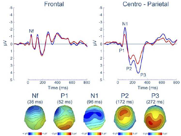
Professor: In Figure 3 are shown the group means for the respiratory-related evoked potential (upper panel) and related scalp topographies at their peak latencies (lower panel), at frontal and centro-parietal regions.

Professor: Also, advanced studies using evoked potentials have identified that most peaks are a composite of different sub-peaks.

Student: Since there are 1,000 ms to a second, all this take place in less than ONE HALF A SECOND.

Professor: And that half a second can be divided into five stages and another stage can be added for producing a subjective report, with the sixth stage taking about another second or so. The following figure illustrate two schemes for the structures and pathways involved:

Schemes

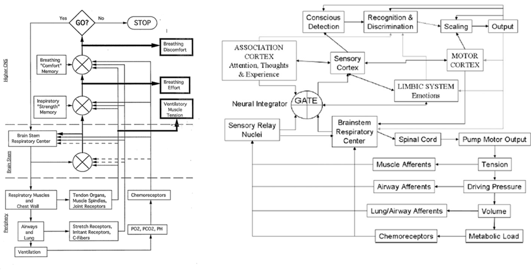
Professor:

• Left figure is from Weiser et al. (1993); notice the three (3)comparators of actual and efference copies, shown as circles with crosses. The resulting three error signals can be self-reported: first, as Ventilatory Muscle Tension; second, as Breathing Effort; third, as Breathing Discomfort.
• Right figure is from Davenport’s contribution to the O’Donnell et al. review (2007). Note the comparator labeled GATE corresponds roughly to the Weiser et al. (1993) comparator for Breathing Effort subjective report.

In six stages

Professor: Below is a model of the time course for sensation processing shown by Figure 5 of Menon & Uddin (2010) with their five stages for processing:

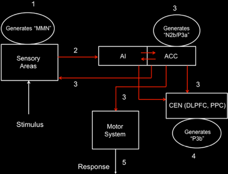
Student: I notice the anterior insula (AI) is tightly connected to the anterior cingulate cortex (ACC), that then influences the central executive network (CEN) composed of the dorsolateral prefrontal cortex (DLPFC) and posterior parietal cortex (PPC). Hmm, “N2b/P3a” is part of the N2 and P3 composite wave and P3b is another part of the P3 wave.

Professor: The numbers in their Figure 5 are the stages of processing. The following are the details for Stage 1:

Stage  1 – At about 150 ms post-stimulus, detection of a ‘deviant’ stimulus by the primary sensory areas, including posterior insula, is indexed by the mismatch negativity (MMN) component of the evoked potential.

Professor:  The stimulus is inspiratory loading, frequently done by a brief inspiratory occlusion, which is a ‘deviant’ stimulus:

• Phrenic nerve activity from pulmonary mechanoreceptor and stretch receptors to
• Cervical spinal cord* and cuneate nuclei*
  • Cerebellum – to lobule V including intermediate cortex* and vermis* via mossy fibers to ventroposteriolateral nuclei and/or
  • Thalamus – to ventroposteriolateral nuclei* from cuneothalamic to fastigal nuclei* to the
  • Thalamic reticular nuclei (TRN)* from the ventroposteriolateral thalamic nuclei and
  • FINALLY TO THE Posterior insula (PI)*.

Professor: For more on efference copies, see my earlier post: Signals-of-efference-copy-and-effort.

Student: Then those asterisks (*) are the possible ‘efference copy comparator(s)’ and/or ‘MMN source(s)’ for

• ventilatory muscle tension,
• breathing effort, and
• breathing discomfort.

Professor: More on ‘efference copy comparators in the coming post on Perceived Exertion. but here are the details for Stage 2:

Stage  2 – Next is a “bottoms-up” MMN transmission to other brain regions, especially anterior insula (AI) and amygdala. AI provides selective amplification of critical, i.e., salient, events that trigger a strong response in the anterior cingulate cortex (ACC).

Professor: This is not too surprising for MMN transmission to quickly go to AI, since the PI and AI are so tightly connected.

• Together, AI and ACC are the critical areas and form the foundation of the Saliency Network (SN).
• In fact, some ‘blocks’ of the AI “play the role of hubs, bridging the anterior and posterior circuits of the insula” (Cauda et al., 2011).
• In addition, both the PI and AI contain “modality-specific primary sensory representations of each of the affective, interoceptive feelings from the body, and that each representation is organized somatotopically in the anteroposterior direction.” (Craig, 2010).

Student: There is also evidence that PI is interceptively oriented, whereas the AI is organized for integration and decision-making (Cauda et al., 2011).

Professor: Onward and outward throughout the cortex. Here are the details for Stage 3:

Stage  3 –At about 200–300 ms post-stimulus, the AI and ACC will have generated a “top–down” control signal, as indexed by the N2b/P3a component of the evoked potential. This signal is simultaneously transmitted to the primary sensory and association cortices, as well as to the central executive network (CEN).

Professor: The alpha traveling wave with the posterior insula’s searchlight finds a focal disturbance and activates the CEN to switch off/reduce the activity of default mode network (DMN).

Student: Oh, I remember! The Saliency Network (see Oops-I-forgot-and-I-must-reconnect-to-the-breath), or the Tonic Alertness Network (see Windshield-wiping-of-cortex-and-using-an-insula-searchlight), ‘sends out an alert’ to the CEN and Sensorimotor Networks as well as dampens the distracting activity of the DMN.

Professor: We’re out of time for this blog post, and the discussion of the next three stages (4 thru 6) will be in the next one:

• Stage  4 – “About 300–400 ms post-stimulus, neocortical regions, notably the premotor cortex and temporo-parietal areas, respond to the attentional shift with a signal that is indexed by the time-average P3b evoked potential.”
• Stage  5 – “The ACC also facilitates response selection and motor response via its links to the midcingulate cortex, supplementary motor cortex, and other motor areas “
• Stage  6 – Subjective report will include “Recognition and Discrimination,” plus “Scaling” shown in Davenport’s 2007 model, plus generation of a verbal report.

Take Home: This post is about the time course of symptom awareness:  Within about .015 seconds, less than one breath, the Saliency Network (SN) of our brain can NOTICE something is strange. At the end of six stages of relatively fast cortical processing, for example, being aware of inspiratory load, we can in the last stage report being “short-of-breath”.

Next: Part 2 will include the last three processing stages also including discussion on generation of symptom report and common neural networks for DYSPNEA, PAIN, and STATIC HANDGRIP.

References

Cauda F, Torta DM-E, Sacco K, Geda E, D’Agata F, Costa T, Duca S, Geminiani G, Amanzio M.  (2011) Functional connectivity of the insula in the resting brain. NeuroImage 55 (2011) 8–23

Davenport PW (2007) Chemical and mechanical loads: What have we learned? In: O’Donnell DE, Banzett RB, Carrieri-Kohlman V, Casaburi R, Davenport PW, Gandevia SC, Gelb AF, Mahler DA, Webb KA. (2007) Pathophysiology of Dyspnea in Chronic Obstructive Pulmonary Disease: A Roundtable. Proc Am Thorac Soc 4: 147–149 – See more at: http://www.endurance-education.com/endurance-education-com/the-lung-airways-are-connected-to-the-stretch-receptors-and-the-etc/#sthash.f7XNPBj7.dpuf

Menon, V. (2010) Large-scale brain networks in cognition: Emerging principles. In: Analysis and Function of Large-Scale Brain Networks. (Sporns O, ed) pp. 43-53. Washington, DC: Society for Neuroscience.

Raux, M., et al., (2013) Functional magnetic resonance imaging suggests automatization of the cortical response to inspiratory threshold loading in humans. Respir Physiol Neurobiol, http://dx.doi.org/10.1016/j.resp.2013.08.005

Sadaghiani S, Scheeringa R, Lehongre K, Morillon B, Giraud A-E, Kleinschmidt A. (2010) Intrinsic Connectivity Networks, Alpha Oscillations, and Tonic Alertness: A Simultaneous Electroencephalography / Functional Magnetic Resonance Imaging Study. DOI:10.1523/JNEUROSCI.1004-10.2010.

Sridharan D, Daniel J. Levitin DJ, Menon V. (2007) A critical role for the right fronto-insular cortex in switching between central-executive and default-mode networks. www.pnas.org/cgr/doi/10.1073/pnas.0800005105.

von Leopoldt A, Chan P-Y S, Esser RW, Davenport PW. (2013) Emotions and Neural Processing of Respiratory Sensations Investigated With Respiratory-Related Evoked Potentials. Psychosomatic Medicine 75: 244-252.

Weiser PC, Mahler DA, Ryan KP, Hill KL, Greenspon LW. (1993) Clinical assessment and management of dyspnea. In: Pulmonary rehabilitation: Guidelines to success. 2nd edition. Hodgkin, J, Bell CW, eds. Philadelphia: Lippincott, 478-511.

 

Part Two

Professor:  This post will continue following someone experiencing a mild pulmonary inspiratory obstruction, like putting on a surgical mask to reduce symptoms of asthma in cold weather. In this post, we will discuss:

• switching attention from being fully alert; to
• planning, selecting, and activating motor responses.

Student: What about:

• consciously detecting and recognizing this event, choosing a verbal description, scaling it, and using the scaled words to report our level of dyspnea.

Professor: Regrets, it’s snow time out here in Pennsylvania, and that discussion will now be in Part 3, the final post of this series.

Student: As a model, we used Figure 5 of Menon & Uddin (2010) with their five stages for processing sensory input and attentional control. The sixth stage we will add about Subjective Report.

Professor: And, what processes were covered during Stages 1 – 3?

Review of Stages 1 through 3

Student: Stages 1 and 2 dealt with being stimulated by our breathing, and definitely these stages were processes that very quickly activated the Salient Network (SN):

• Stage 1: CONTACT has been made.
  • About 150 ms post-stimulus, the primary sensory areas, including posterior insula (PI),
  • detected ‘deviant’ local activities.
  • Stage 2: So, WAKE UP!
    • Within several more milliseconds, a “bottoms-up” amplified signal was quickly transmitted to other brain regions, including the anterior insula (AI) that
    • then triggered a strong response in the anterior cingulate cortex (ACC).

• Stage 3: Executives, Shift to Fully ALERT!!!!
  • About 200 – 300 ms post-stimulus, the SN sends out “top–down” control signals to the central executive network (CEN) as well as
  • to the default mode network (DMN).

Review of Networks’ Nodes Discussed So Far

Professor: First, I want to make sure we are all clear about the SN, CEN, and DMN networks by reviewing their actual pathways and concentrating on the pivotal role of the insula:

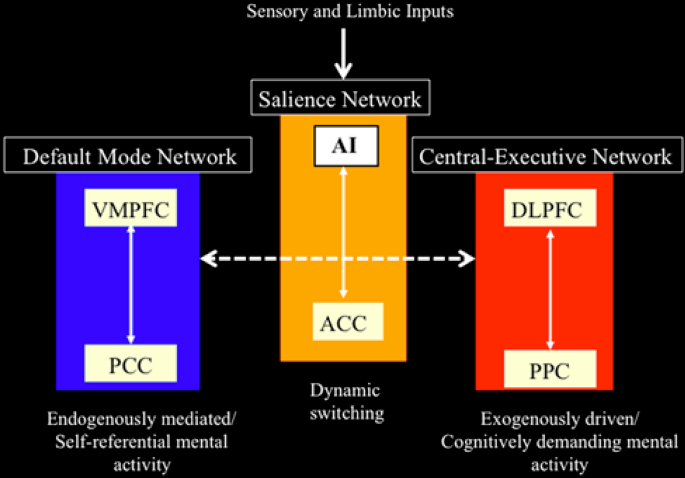
Professor: Above is Figure 4 from Menon & Uddin (2010). It is their network model that highlights anterior insula function. To paraphrase their figure legend:

• the AI is a node for the salience network, working closely with the ACC SN node;
• the AI and ACC intensely initiate dynamic switching between the CEN and DMN; and
• notice at the very, very top of the Menon & Uddin model, that the inputs arrived from sensory and limbic systems and are initially processed by the anterior insula (AI).

Professor: I want to add some more details about the CEN, DMN, and other networks:

• Two lateral cortex areas locate the nodes of the CEN:
  • the dorsal lateral prefrontal cortex (DLPFC) and
  • the posterior parietal cortex (PPC),
  • Two medial cortex areas locate the nodes of the DMN:
    • the ventral medial prefrontal cortex (VMPFC) and
    • the posterior cingulate cortex (PCC), and
    • Other distributed neural circuits comprise “task-specific” networks.

Student: Hey! Colorful pictures. Thanks for putting these detailed illustrations of the neuroanatomy and actions for these areas down at the bottom of this post (Go to see these cortical areas).

Professor: I hope they are helpful for the ‘out-of-the-loop’ folks. Now, after about 200 – 300 ms post-stimulus, our mind has shifted its attention and is ready for action/reaction during the upcoming Stage 4:

Stage 4: Higher cortical regions, especially the premotor cortex along with the temporo-parietal areas, respond to this attentional shift.

Professor: Basically, the control signals from DLPFC and PPC of the central executive network ‘turn off’ the cognitive activities of the VMPFC and PCC of the Default Mode Network. Menon & Uddin (2010) have reviewed a study using a specific task to provoke increased CEN activity accompanied by decreased DMN activity.

Student: Please tell me more about this task!

Professor: It was an “oddball” task that was utilized by Sridharan et al. (2008):

• it involved the detection of an infrequent blue circle embedded within a sequence of many, frequent green circles and presented in the center of the black screen;
• their results suggested that rAI was tonically alert for the infrequent colored circle; and
• NOTICE that in this task there was a different colored circle.

Student: That is a weird kind of an oddball!

Professor: Let’s turn to Figure 3 in the review of Menon & Uddin (2010) and discuss the information flow during this “oddball” task. These streams are among the major nodes of the salience, central executive, and default mode networks.

Review of Networks’ Nodes Discussed So Far

Professor: First, I want to make sure we are all clear about the SN, CEN, and DMN networks by reviewing their actual pathways and concentrating on the pivotal role of the insula:

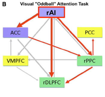
Professor: Above is their Part B of Figure 3. The Saliency Network has blue filled rectangles; the Central Executive Network has green filled rectangles; the Default Mode Network has yellow filled rectangles; active outflows are red arrows; inactive outflows are gray arrows.

Professor: As emphasized in their Figure 3 legend, only the right AI (rAI) had a large excitatory outflow to its companion  ACC nodes. Also, rAI inhibitory had outflows to the CEN’s rDLPFC and rPPC nodes. The activation of ACC also reinforced inhibition of the rPPC. These connection analyses, together with latency analyses, suggested to Menon & Uddin (2010) that the rAI:

• “functions as a “causal outflow hub” for the detection of critical, salient events and
• “initiates network shifting.”

Professor: However, this was certainly an “oddball” lab study. An actual situation was studied by Hasenkamp et al. (2012):

• who also confirmed the results of Sridharan et al. (2008) and
• who had participants ‘be alert for any mind wandering’ and then make a shift back to a sustained focus :

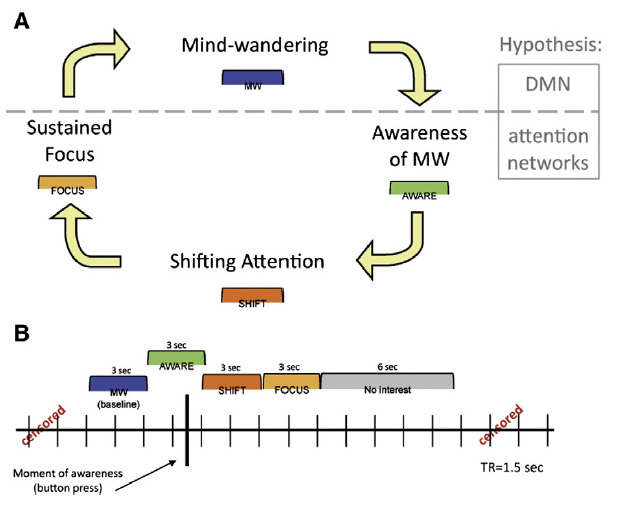
Professor: The legend for Figure 1  indicated that Panel A has a horizontal gray dashed line representing a hypothesized division between DMN and task-positive attention network activity during these states. Panel B is a model for the construction of phases relative to the button press (represented by the heavy black vertical line).
Professor: In this study, the only thing the participants had to do was to lie down in a MRI scanner and try to meditate on breathing in and out. Figure 1 above indicates that:

• the key task was to NOTICE when one was not attending to the object of meditation, i.e., on  THE BREATH; and
• at the moment of ‘awareness’ they pressed a button.

Student: I just re-read your August 1, 2013 post, I-must-reconnect-to-THE-BREATH, and here is my summary of the phrases:

• Oops: In the 3 seconds containing the button push, i.e., the AWARE phase (that was when a MRI scan contained the button push) the active areas were chiefly in the midbrain, left posterior insula and, of course, the SN.
• Sent out the Alert: In the SHIFT phase, the CEN and subcortical areas became active.
• Keep on keeping on: During the FOCUS phase, activation persisted within the CEN’s right dorsolateral PFC, but only in this brain region, perhaps to maintain sustained attention on THE BREATH.
• Being Distracted: Sometime later, the MW phase was associated with activations in the DMN areas, perhaps used for internal thinking/day dreaming and, in addition, the ‘motor’ preparation areas for the button push.

Student:, I have encouraged others to look at the MRI illustration for these stages. In fact anyone could click this link, , I-must-reconnect-to-THE-BREATH, and read about this important study.

Professor: Thanks, and of course, the key to all these studies is the word ATTENTION. Now, in our example, discomforting breathing has gotten our full attention; in order to consider what action to take, and, in deciding whether or not to do it, we will be using the activities of Stage 5:

Stage 5: The ACC also facilitates response selection and motor response via its links to the midcingulate cortex, supplementary motor cortex, and other motor areas.

Professor: Still getting hard to breathe, eh? Well, your motor networks can help you:

• keep on doing what you are doing, or
• freezing, or
• taking action by doing something else.

Student: Right now, I think it’s time to take two puffs from a medication inhaler, the one I use for treating bronchospasms.

Professor: A great opportunity! Let’s have our example take place where you can make a visually-assisted grasping of your inhaler.

Student: Well, let’s say that the inhaler is on a dresser in my bedroom, and I could either:

• hop over my bed to grab it, or
• walk slowly around my bed to pick it up without getting any more short-of-breath.

Professor: And you get to make a choice! The review of Cisek & Kalaska (2010) can help specify, select, execute, and fine tune your route.

• They reviewed how monkeys and humans decide what movement to do and how to do it, and
• they even illustrated their review with the data, results, figures, and conclusions from the amazing study of Ledberg et al. (2007), that
  • uses simultaneously recorded, local field potentials from multiple sites across the brain of awake, behaving monkeys
  • while they perform a very similar conditional Go/NoGo task, pressing and choosing whether or not to release a lever.

Student: I do act like a monkey some times.

Professor: Therefore we can substitute the suggested neural mechanism from the review of Cisek & Kalaska for a monkey’s visually-guided reach-and-grasp task that is shown below:

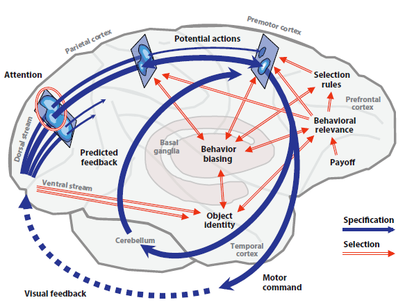
Professor: Note their figure 1 shows our primate brain, emphasizing the cerebral cortex, cerebellum, and basal ganglia. Their figure legend is expanded with my comments below:

• At the far left, the monkey’s eyes feed information into the beginnings of the parallel processing and diverging dorsal and ventral streams in the visual cortex.
• Dark blue arrows are the dorsal stream,
  • represent the processes of action specification, the “what to do” pathways, which
  • transform visual information into neural representations of several or many potential actions.
  • Blue ovals on rectangles portray the representations for three neural populations along this dorsal route.
  • Ledberg et al. (2007) confirmed that a very fast, feedforward sweep, of evoked potential activity, that was stimulus onset-related, occurred
    • within 55–80 ms in the frontal eye fields and premotor cortex via the dorsal stream and
    • within 50–70 ms in the visual cortex via the ventral stream.

Student: Those neural circuits are really ‘fast out of the starting blocks’!

Professor: This seems to hold for any reactive task. At this point, both the dorsal and ventral streams are transmitting information to each other, concentrating on clarifying action specification. The following  paraphrases the Figure 1 legend of Cisek & Kalaska (2010):

• Notice that each of the three neural populations is depicted as a map
  • where the lightest regions correspond to peaks of tuned activity, and
  • which then compete for the final action specification.
  • Red double-line arrows are the ventral stream
    • that represent input from the initial visual cortex and
    • input from the basal ganglia and prefrontal cortical regions,
    • that collect and process additional information for final action specification,
    • This information sharing that occurred somewhat later with the dorsal stream circuitry providing biasing selection:
      • discerning information about motor output parameters like direction of different stimulus categories,
      • happening within approximately 100 ms of onset in visual association areas of the monkeys and
      • within 200 ms in their prefrontal sites.

Student: No anxious hesitation is happening when monkeys have full attention on its task performance!

Professor: Finally this visually-guided movement selection utilized computations of object identity, assessment of behavioral relevance, and prefrontal rules for a final action specification, i.e., “winner-takes-all.”

• The monkey’s Go/NoGo decision processing
  • appeared approximately 150 ms after stimulus onset and
  • occurred nearly simultaneously, within a diverse interacting “mosaic” of cortical sites, including visual, motor, and executive control areas, until
  • it resulted in the post-decision subprocesses that were involved with coordinating the final motor execution.
  • The selected action is ‘disinhibited into execution’ (i.e., “GO!”) and is then fine-tuned by:
    • external, overt feedback from the environment (dotted blue arrow), as well as
    • internal reafference , i.e., collateral, predictive feedback provided by the cerebellum.

Student: Then, how fast does all this take place?

Professor: It takes less than 0.3 s, i.e., less than 300 ms, for the overall reaction time to release the lever.

Student: Wow! All that just to release a lever or not.

Professor: To release or not! I wonder if you are you inferring that there is another final gate involved. And YES, states Hanakawa (2011), with his notion of a “firewall-like” rostral premotor gateway.

 

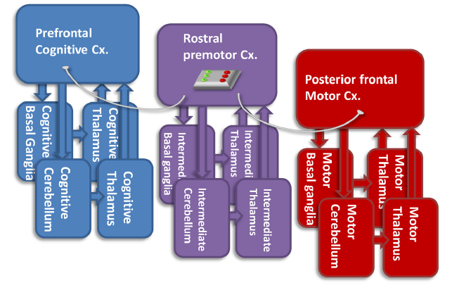
Professor: Above is his challenging Figure 3. Briefly, it is his hypothetical view of the functions of the rostral premotor-subcortical network (Cx.) for connecting the prefrontal cognitive and the posterior frontal motor networks. He recognizes that:

• the “pure motor” posterior frontal network has direct connections with the spinal cord,
• but it does not directly interconnect with the “cognitive” network.

Professor: Hanakawa suggests that one of the functions of the rostral premotor-subcortical network may be gating, i.e., connecting/disconnecting the cognitive and motor networks, depending on the context.

Student: Well, then the rostral premotor-subcortical network acts like a Motor Gate, just like the Thalamic Reticular Nuclei act like a Sensory Gate!

Take Home: So far, we have learned about turning our attention fully to our uncomfortable breathing and using visually-guided reaching to get a inhaler. Now how do we verbally communicate the effect of taking the bronchodialator from the inhaler?

Next: Stage 6: Subjective Report is the next and final stage of perceptual processing post for this blog.

References

Cisek P, Kalaska JF (2010) Neural mechanisms for interacting with a world full of action choices. Annu Rev Neurosci 33: 269–98. doi: 10.1146/annurev.neuro.051508.135409.

Hanakawa T. (2011) Rostral premotor cortex as a gateway between motor and cognitive networks. Neurosci Res70: 144–154. doi: 10.1016/j.neures.2011.02.010.

Hasenkamp W, Wilson-Mendenhall CD, Duncan E, Barsalou LW. (2012) Mind wandering and attention during focused meditation: A fine-grained temporal analysis of fluctuating cognitive states. NeuroImage 59: 750–760. doi: 10.3389/fnhum.2012.00038.

Ledberg A, Bressler SL, Ding M, Coppola R, Kakamura R. (2007) Large-scale visiomotor integration in the cerebral cortex. Cereb Cortex 17 (1): 44-62. doi: 10.1093/cercor/bhj123.

Menon V, Uddin LQ. (2010) Saliency, switching, attention and control: A network model of insula function. Brain Struct Funct 214: 655–667. doi:10.1007/s00429-010-0262-0.

Sridharan D, Daniel J. Levitin DJ, Menon V. (2008) A critical role for the right fronto-insular cortex in switching between central-executive and default-mode networks. Proc Natl Acad Sci USA. 105: 12569–12574. doi/10.1073/pnas.0800005105.

Last Part

Professor:  This post will finish the proposed six (6) stages for handling breathing discomfort. So far, we have completed a tour through the first five (5) stages:

Edit

1.	CONTACT!	A breathing alarm signal just arrived at posterior insula!
2.	SEND OUT ALERT!	Anterior insula and the rest of saliency network (SN) received the alarm, too!
3.	FULL ATTENTION!	The SN puts the Central Executive Network on the lookout & quiets down the Default Mode Network!
4.	GET READY TO ACT!	Task: Breathing ‘tubes’ want medication via inhaler!
5.	ACT!	Action: Go get inhaler and use it!

 

Professor: We will add a final, sixth stage for communication to Menon & Uddin’s model of perceptual processing (2010) that has been our guide for the first two parts. (Here are links to Part 1 and to Part 2.)

 

Edit

6.

COMMUNICATE!

Let others know how well the medication is working!

 

Professor: This sixth stage estimates, not produces, a subjective rating of shortness of breath. For example, “Easy breathing” or “It’s moderately hard to breathe!”

Student: Some people ask me about my breathing. And I really don’t know what to say!

Professor: Asking questions is great tool for opening our ability to connect to our self. Already our mind has shifted its attention and is taking actions. Talking about symptoms, while experiencing them, is in the details for the upcoming Stage 6:

• Stage 6: Communicate!
  • Use the steps for seeing or hearing a question being asked about symptoms, and then
  • take the steps for answering the question.

Student: So, therefore we are constantly processing some sort of input, coming into our ears or eyes and even appearing from our self-talk.

Professor: All this processing is a combination of important activities for our constantly, tonically alert, saliency network.

Student: To make our discussion easier, let’s pick a rating scale based on simply hearing a question!

Professor: Yes, I will emphasize ‘hearing.’ In fact, using our old verbally administered scale, the 0 – 10 dyspnea scale, one can:

• first, hear a question, like “What’s your dyspnea number?”;
• second, understand the question is about severity of breathlessness;
• third, decide on the appropriate description from a dyspnea scale;
• fourth, retrieve the dyspnea scale number for it; and
• fifth, out loud, say the number.

Student: Perhaps, we could use a scale like the rating of perceived exertion (RPE), as a breathing discomfort scale, that ranges from zero for “not at all uncomfortable” to 10 or more for “severe discomfort.”

Sound to Meaning

Professor: Years ago, my colleagues and I used this 10-point scale (Borg, 1982, 1999) to better understand dyspnea (Weiser et al., 1993). However, to start investigating “sound to meaning,” (borrowing a phrase from Hickok & Pöppel, 2007), coming up is a mental picture that is worth a thousand words.

Student: Please keep it simple.

Professor: Okay. According to Price (2012), “The landmark of functional imaging [studies] of auditory and visual word processing was published in 1988 by Petersen and colleagues who used” positron emission tomography (PET)

• “to identify the brain areas activated when healthy participants
• “were presented with auditory or visual single words and
• “were instructed either to view them passively, repeat them or generate a verb that was related to the heard or seen noun (e.g. “eat” in response to “cake”). “
• Based on the results, “the authors concluded that:
  • “auditory word forms [involved] the left temporo-parietal cortex,
  • “visual word forms [involved] the left extrastriate cortex,
  • “semantic associations involved the left ventral prefrontal cortex,
  • “word generation involved the [bilateral] dorsolateral prefrontal cortex;
  • “general response selection involved the [bilateral] anterior cingulate;
  • “articulatory coding and motor programming involved the left ventral premotor cortex, left anterior insula … and supplementary motor cortex (SMA) and
  • “motor execution involved the rolandic cortex (the posterior part of the precentral gyrus bordering the central sulcus).”

Professor: Price concluded that, “the results provided a new anatomical model of lexical processing (Petersen et al., 1988; Petersen et al., 1989) that is illustrated in [the figure below].”

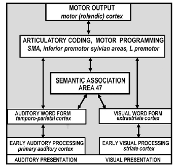
Professor: According to Price (2012), the key features of their model were,

• “the inclusion of a small number of discrete areas
• “with multiple parallel pathways [split between auditory and visual]
• “[among] localized sensory-specific, phonological, articulatory and semantic-coding areas.”

Student: Ahha. I believe that “The Magic of Listening” is beginning to make sense.

Professor: Since the front-end of speech is listening and comprehending, it is like paying attention to a phone answering machine. And the ‘speech stream’ for listening begins with the processing of words and sentences from the ‘voice message.’

• This stream begins with both ears and quickly is communicated to the BILATERAL middle and posterior superior temporal lobes.
• It involves preprocessing by medial geniculate nuclei of the thalamus, insula, amygdala, and cerebellum.
• It happens extremely fast.
• And it begins with a ‘mismatch negativity’ (MMN).

Student: Thalamus again! Insula again! MMN again! This is beginning to sound like a recurring, primitive, perceptual theme song.

Professor: You betcha. And Specht (2014) reminds us that the primary and secondary auditory cortices

• “belong neither to the ventral nor to the dorsal stream, as they provide general auditory processing capacities, which is important for both streams (Hickok and Poeppel, 2007)” and
• “are assumed to send output to the middle and posterior” superior temporal sulcus (STS), “from where the two neural streams may originate (Hickok & Pöppel, 2007; Turkeltaub & Coslett, 2010).”

Student: Enough words! Give me a neuroanatomy picture!

Professor: Below is Figure 1 from Rauschecker & Scott (2009) illustrating what happens when a monkey sees lightning and hears thunder:

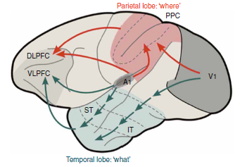
The abbreviations are, in order of activation:

• V1, primary visual cortex (from seeing lightning);
• A1, primary auditory cortex (from hearing thunder);
• IT, inferior temporal region (processing visual perception);
• ST, superior temporal region (processing audio perception);
• PPC, posterior parietal cortex (associations for audio-visual perception);
• DLPFC, dorsolateral prefrontal cortex (executive functions of ‘where:’ spatial relations and action); and
• VLPFC, ventrolateral prefrontal cortex (executive functions of ‘what:’ selection and retrieval semantic/linguistic knowledge).
• Red is for dorsal stream and
• green is for ventral stream.

Professor: Figure 1 from Rauschecker & Scott (2009) shows a simple, dual processing, audiovisual scheme with ‘what to do’ in blue and ‘how to do it’ in red.

• It clearly illustrates the paths of the monkey ‘processing gradient’ in the temporal lobe.
• Research findings indicate that increasingly complex processing is done more anteriorly.
• In addition, the lower, ventral stream is shared rather than split;
  • the left hemisphere stream deals more with speech comprehension, and
  • the right hemisphere stream handles prosaic and personal identity information.

Student: Say! These dorsal-ventral streams seem like visual-assisted motor action. Perhaps these pathways are another example of “form follows function,” since they are like the ones for grasping the medication nebulizer!

Professor:  Yes, indeed! It’s more like ‘audio- visual’-assisted motor answering. First of all, concerning language, our mind uses these pathways to find FAMILIAR words occurring within questions and other sentences that we hear, as shown at the bottom of the following figure:

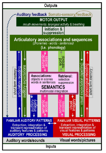
Professor: Above is a more complicated figure 2 from the review of Price (2012). It adds recently defined, functional terms to the basic speech processing model proposed by Petersen et al. (1998. 1999) and is shown near the beginning of this post. It begins with extraction, integration, and transient representation of words in our question, “What is your dyspnea number now?”

Student: Hmm. Do we actually tear apart the ‘noise of voices’ so that we can reassemble their gibberish parts into a meaningful question?

Professor: Yup. We disassemble and then loop through the segments to reassemble their speech for our comprehension. To understand this, Tyler & Marslen-Wilson (2008) suggest the following sub-system approach:

• first, word morphological processing, especially verb inflections for tense and gender,
• then, sentence-level syntactic processing, and
• finally, sentence-level semantic processing.

Processing of Word Forms

Professor: To repeat, many word segments are frequently heard and become FAMILIAR ones, or some are INFREQUENTLY heard so that they render a segment to be AMBIGUOUS. If ambiguous, then additional processing will be required.

Student: Do I have to hear every segment and only react if it is not familiar?

Professor: No, not at all. Fortunately, we are ‘proactive’. It seems that we are continually ‘looking ahead’ anticipating what we are about to hear (see Borovsky et al., 2012; Dikker & Pylkkanen, 2014). Part of this predicting is quickly ‘asking ourselves,’ “TO PARSE OR NOT TO PARSE?”

• That is, if these words are not matched in our mental lexicon which is located in the temporal lobe, then parse. Some examples are:

Edit

for nouns, verbs, etc.:	“numver”	instead of “number”
for names:	“Paul Wiser”	instead of “Phil Weiser.”

• For nouns and verbs. When “numver” was not found with temporal processing, that information is sent to the IFG and used by a comparator circuit to find
  • any stem, like “pump” or “jump,” and
  • any ending (affix) like “er” or “ing.”
  • Then when the stem “numv” was not found with temporal processing, then an area in the IFG, the left posterior opercularis (LpOp), did a search of its mental lexicon for a representation and “numb” was found.
  • So there you have it: therefore, it was a misspelling, and a ‘recoding’ was done back into the reconstructed pSTS sting, creating the word “number” in neural terms.
• For names. For me, my LpOpmental lexicon has both ‘frequently said’ words and printed words that are associated with this web site. In our example, this CONTEXT helps when I am
  • doing a search, perhaps using some sort of comparator circuit in my IFC,
  • using first letter of “P” or “W” and last letter of “l” or “r,” that results in
  • finding “Phil” and “Weiser,” and
  • performing another ‘recoding’ of these two names.
• Then these matched or nearly matched nouns, verbs, names, etc. are added to temporal lobe working memory.
• This looping routine of “parse or not to parse” is continued until it is finished with the word’s last sound segment.

Professor: If you want more details of structures involved in resolving highly ambiguous words or sentences, read Price’s review published on 2012.

Student: Hmm. Therefore, words are broken down into segments, compared to anticipated, familiar, stored traces, and the ‘best choice’ is selected for reconstructing the question or sentence.

Syntactic Processing of Sentences

Professor:  Yes, indeed. The processing described for words can be extended to questions and other types of sentences.

• In fact, syntactic processing reveals the arrangement of words and phrases in a sentence and determines whether or not it is ‘well-formed.’
• “The core human capacity of syntactic analysis involves a left hemisphere network involving left inferior frontal gyrus (LIFG) and posterior middle temporal gyrus (LpMTG) and the anatomical connections between them,” state Tyler et al. (2013).
• Our sentence is, “What is your dyspnea number now?”
  • Fortunately it is an uncomplicated one to hear and understand.
  • A more complex one could start with, “In the circus juggling knives ….” And so far, this phrase does not hint at what will come next.
  • Will it become “In the circus juggling knives is less dangerous than eating fire.”? or
  • might it become “In the circus juggling knives are less sharp than people think.”?

Student: Therefore, it’s when you hear “is” or “are” that the phrase “juggling knives” is clarified.

Professor: So it was these two sentences and others that Tyler et al. (2013) used to clarify sentence syntactic comprehension.

• They utilized MEG to record the time course of disambiguation and found changes in activity for the LpMTG and LIFG.
  • The words “juggling knives” comprised their “central phrase” and “is” or “are” was the disambiguating word.
  • They characterized how syntactic information for different items changed over time.
• Results:

Edit

Event	R/L pMTG	LIFG
“juggling” spoken	Nothing	Nothing
“knives” spoken	Lexico-syntactic representation of first word of central phrase that assumed it preferred a direct object as the second word. Ambiguity of central phrase is established after integrating the first and second words; second word was not a direct object.	Nothing
“is” spoken	The pMTG represented the remaining incoming speech and sends the disambiguating phrase representation to the LIFG. Maintains representation of the form of the incoming speech and updates the interpretation of the central phrase and how well-formed the central phrase and disambiguating verb ‘sound.’	LIFG representation only reflects ambiguous items from LpMTG, i.e., those items with multiple meanings. Revised second word as a subdominant and resolved the ambiguity; transmited revised property for second word to pMTG.

Professor: Then the syntactic process loops through the rest of the question or sentence.

Student: By the way, what’s the difference between syntactic and semantic?

Semantic Processing of Sentences

Professor:  Let’s look at how well organized a sentence may be.

• If it is well-formed, then all the rules of syntax are obeyed and it ‘flows’ easily.
• However, if the sentence is, “I just ate a cloud.” it might ‘flow’ easily, but it is ill-fitting with one’s knowledge of the world” (Pylkkänen et al., 2011).

Student: Therefore, the sentences should be both well-formed and well-fitting!

Professor: Correct! Semantic processing will reconstruct the entire sentence, word-by-word, into a personally meaningful statement that is drawn from one’s knowledge of or beliefs about the world (from Pylkkänen et al., 2011).

Student: Then, how does my ‘language mind’ know if the well-formed question, “What is your dyspnea number now?” is also well-fitting?

Professor: Well, first of all, semantic processing is highly coupled to syntactic processing. However, by adding some more semantic complexity we could force a decision about ‘fit.’

• Brennan and Pylkkänen (2010) suggest analyzing a more complex sentence that is, “The child cherished the precious kitten.” This sentence is actually semantically confusing and mentally a bit difficult to quickly interpret.
  • since it implies an unusual, unchanging state for the noun phrase “kitten,” an animal which is usually doing something,
  • whereas the verb phrase “began to cherish” will fit with a changing state for the child.
  • Instead,the ‘subconscious sentence’, “The child began to cherish the kitten,” would be very fitting.
• For an on-line resolution, these linguists suggest adding a ‘change-of-state’ phrase “(with)in a ….”
  • So the incomplete sentence becomes “Within a few minutes, the child cherished the kitten.”
  • And our mind will quickly ‘coerce’ it to be interpreted as, “…the child [came to cherish] the kitten.”

Student: Hey! How did our mind do this?

Professor: These investigators timed how long subjects took to read unresolved statements and then monitored the MEG of another group as they read the same statements. The results were:

• incomplete statements took longer to process,
• and the MEG showed increased activity at about 300 ms after presentation of the verb, e.g., “cherished” for
  • ventromedial Prefrontal Cortex (vmPFC) and
  • left anterior temporal lobe (LaTL).

Professor: Brennan and Pylkkänen (2010) suggested that the primary loci for basic combinatorial processing are the

• vmPFC for computing the most likely semantic structure and
• LaTL for reconstructing the inferred syntactic structure.

Student: Therefore, the more complex segments are processed in the ventromedial prefrontal cortex and the anterior areas of the temporal lobe, including the temporal pole, until word parsing has completely finished handling the entire sentence.

Professor: Now let’s ‘find’ the meaning of our sentence, “What is your dyspnea number now?” Perhaps its meaning becomes more understandable as its words are processed as shown in the table below:

Edit

Word	Meaning	Sound Stress
What	a question’ => ‘tell me about’	Higher
+ is	‘something equals something’	Lower
+ your	‘my’	Also low
+ dyspnea	‘uncomfortable breathing’	Highest
+ number	‘intensity’	Low
+ now	‘at this time’	Higher
All together	Tell me a number for your uncomfortable breathing.

Student: Its category is a question and interpreting its meaning looks easy.

Professor: Yes. All that’s requested is choosing a dyspnea scale descriptor, selecting its number, and saying that number out loud.

Sound to Action

Professor: Of course, the flip-side of listening is answering. Our question is, “What’s your dyspnea number now?” The answer could be, “My dyspnea number is […].”

• This is the ‘back-end’ of speech processing, i.e., speech production.
• And the phrase “sound to action” is also borrowed from Hickok & Pöppel (2007).
• In fact, Price (2012) cites Papathanassiou et al. (2000) stating, “The processing involved in speech production overlaps with that involved in speech comprehension.”
• In producing speech, basically we will reverse some of the processes that were involved in speech comprehension.

Student: Whoa! To produce an answer, all I do is reverse the speech comprehension process?!

Professor: Of course. Let me check what my thinking and speaking actions might be to estimate the magnitude of my dyspnea sensations. I will examine a personal experience estimating shortness-of-breath (SOB):

• I am running on a treadmill at 9.25 mph up a 2 % grade, with lots of wires hanging off me for forty minutes now, with twenty minutes to go.
• An experimenter tells me it’s time to choose a SOB number.
• I ‘see’ the Borg 10 point scale in my mind’s ‘eye’ even though it is hanging in front of me.
• My choices are to
  • repeat the prior number since this is a time series experiment, or choose a new number.
  • Since my SOB estimate has increased from ‘somewhat severe’ to ‘severe’ dyspnea, I pick the scale number for the new intensity: 5.
• Now I use my articulatory motor system for to say “5″ out loud.

Student: As a scientist, how does your brain estimate magnitude ?

Professor: That’s quite a very provocative question. Think of a burner on a stove and putting your hand high over it. Your hand might feel somewhat warm, and as I turn up the burner heat, you could say that, “Now the skin on my palm is beginning to feel very warm. In fact, I am pulling my hand away.” You just used magnitude estimation!

Student: But how do you estimate the magnitude for this thermal challenge and also for dyspnea attacks?

Professor: Surprisingly, pain and dyspnea activate mostly the same cortical networks. Von Leopoldt and co-workers (2009) published an amazing study contrasting the stress of

• breathing through an inspiratory resistance versus
• coping with heat pain via a temperature sensor placed on skin just below the sternum.

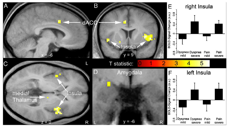
Professor: Fig. 3 in their article shows brain activations during the perception of dyspnea and pain. Their conjunction analysis of the BOLD signals

• demonstrated an increase of activity in the insula from:
  • mild to severe dyspnea (upper right panel) as well as mild to
  • severe heat pain (lower right panel) and
• revealed common activations during perceived dyspnea and pain in the
  • left dorsal anterior cingulate cortex (dACC, part of the Semantic Network),
  • bilateral anterior/mid insula (part of the Semantic Network),
  • right medial thalamus (part of the Brainstem Network), and
  • left amygdala (part of the Brainstem Network).

Professor: The investigators concluded that the discomfort from dyspnea and thermal pain activate common human brain network, and this brain activity seems to correspond to Stages 1 and 2 for the sensation processing model of Menon and Uddin (2010).

Student: Therefore, we have another example of the posterior insula’s SEARCHLIGHT function seeking out unpleasant sensations, in this case, breathing discomfort, which will be transmitted to the anterior-mid insula. Curiously, do the posterior and anterior insula ‘belong’ to two different networks?

Professor: Yes indeed! In fact, this separation is shown by many recent studies. All had the same conclusion in spite of using different pain stimuli:

• Oertel et al. (2012) – puffs of CO₂ (an acid stimulant) to the left nostril,
• Lin et al. (2013) – electrical stimulation of the enamel of right upper incisor, and
• Pomares et al. (2013) – laser stimulation to the radial dorsum of the left hand.

Professor: This separation is clearly shown in an elegant two part study done by Cauda et al. (2014). They utilized both pin-prick pain and touch non-pain stimulation and then applied a “fuzzy” analysis to identify clusters for both groups. This technique performed a parcellation of “each voxel’s time course in a time window of [only] 22 s after the stimulus presentation.”

Student: Brilliant! In their results, they state that, “The percentage of stimulus-locked brain voxels detected by this clustering method was 39%, while the [General Linear Model (GLM)] method only showed 23% of the brain voxels as active.”

Professor: They named these clusters: Posterior Insular, Cingulo-[Anterior] Insular, Fronto-Parietal, DMN, Visual, and Somato-Motor. Below is Figure 5 from their article:

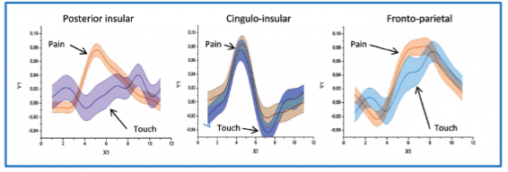
Professor: The figure for Cauda et al. (2014) shows the time-locked, event-related averages for the “clusterization results.”

• “[This panel shows] the comparison between the temporal profiles of the 3 positive clusters of the touch experiment and the correspondent cluster of the pain experiment.
• “The Posterior Insular cluster clearly activates differently for pain than for touch; the other two clusters showed similar responses.”

Student: Here is another ‘conserved’ form, one concerning noxious stimuli. But how do we ESTIMATE MAGNITUDE?

Professor: Well, the mechanism for MAGNITUDE ESTIMATION is a bit of a mystery for me. Maybe the recent, very well-designed, experiment done by Baliki et al. (2009) might provide some clarification. They

• obtained ratings for thermal pain during a fMRI scan and
  • used the ratings to create lines on slides that were then
  • rated as visual lengths by the same participants during a separate scan,
  • which unknown to them were varying in length with the pattern of their ratings of the thermal stimulus;
  • in effect they were doing a quasi-replication, i.e., a rating of a rating.
• Participants used a finger-span device to rate changes in thermal pain and bar length.

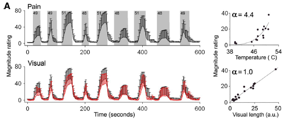 Professor:  Above is Panel A of Figure 1 in the Baliki et al. article showing the average ratings made on the participants.

• Top: The gray areas delineate epochs and intensities of the thermal stimuli with the
  • the black trace showing the average heat pain ratings (bars are SD).
• Bottom: The black trace is the visual stimulus obtained from the subject’s pain ratings, and
  • the red trace corresponds to the average length rating [of the ratings] for the same subjects (bars are SD).
• Right: Scatterplots show the relationship between stimulus intensity and perceived magnitude that
  • follows a power function with exponent of 4.4 for pain and 1.0 for visual ratings.

Student: Looks like classical psychophysics to me, but how do we ESTIMATE magnitude?

Professor: Hang on to your hat! Here come some hints for the MAGNITUDE ESTIMATION mechanism.

• Most importantly, Baliki and co-investigators wanted to know
  • how spread out were the ratings per subject; that is, how much magnitude variability there was in their ratings; so they
  • calculated the variance for the pain ratings and for the visual length ratings.
  • Note the experimental design stresses that the average variance of pain and length ratings will be the same, since the length rating is ‘a rating of the pain rating.’
• Then they performed a whole-brain, voxel-wise, conjunction analysis to find areas that shared the same patterns of the mode-independent variance in ratings and found associated activity in
  • magnitude-specific areas of the bilateral insula, that they termed mag-INS, and also in the
  • bilateral dorsal premotor cortex, ventral premotor cortex, posterior parietal cortex, and middle temporal cortex, with midline activations in mACC and SMA.
  • Note that these regions are found only in the cortex.
• This conjunction analysis was based on analyzing regions of interest (ROIs) that were
  • defined from the random effects analysis of or the pain & visual conjunction map (task-common regions) and
  • delineated using an automated anatomical parcellation labeling procedure.

Student: They struck GOLD! Yes, the magnitude-specific areas of the bilateral insula (mag-INS) store the intensity of pain sensation!

Professor: What concerns us most is MAGNITUDE, and that is all that matters for the conjunction analysis.

• It ignores that the rating was either of pain or of length; all that mattered was size of the rating, independent of these modalities.
• The mag-INS and all the other associated areas were strictly in the cortex, perhaps being network of sorts for estimating and storing MAGNITUDE.

Professor: Finally Baliki and co-workers performed a contrast analysis to compare the pain- to visual-task ratings and then correlated them with the ROIs that encoded task variance and

• found that this pain-specific activity was in the
  • other special areas of the bilateral insula, that they termed noci-INS, and also in the
  • bilateral amygdala, thalamus, basal ganglia, and ventral striatum.
  • Note that these regions are found below the cortex in subcortical areas.
• This analysis began with
  • using the visual length-task ratings as the baseline for
  • calculating the additional amount of activity specifically associated with pain.
  • Finally they performed a contrast analysis comparing the group average visual- and pain-ratings with the ROIs encoding pain-specific activity.

Student: Picture! Picture! I want to see these parts of the insula.

Professor: Below is Figure 4 from Baliki et al. (2009) showing the brain regions encoding magnitude and the brain regions encoding pain sensation.

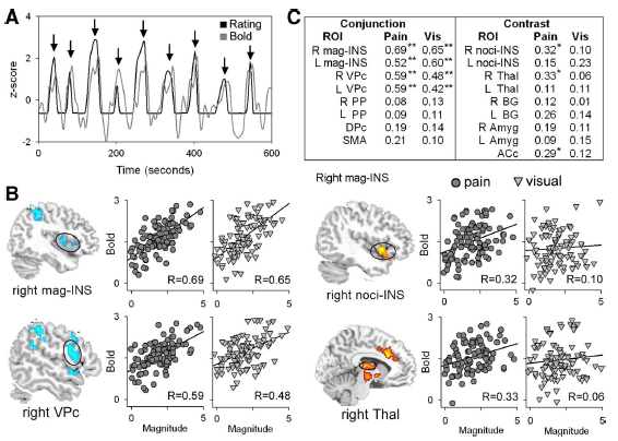
Professor: Below are excerpts from the legend for Figure 4.

• Panel A: Example of blood oxygenated level dependent (BOLD) signal and rating in standard units (z-score) from one subject. Peak BOLD and ratings were
  • extracted for each stimulation epoch (indicated by arrows).
• Panel B: Correlation of BOLD with magnitude for 2 regions derived from the conjunction of variance-related values (blue) and for 2 regions derived from contrast values (red).
  • Scatterplots depict the degree of association between individuals’ region of interest (ROI) signal and magnitude for pain (circles) and visual (triangles) stimuli.
  • The ordinate represents functional magnetic resonance imaging (fMRI) signal and the abscissa represents the magnitude rating for each stimulus epoch for each participant.
• Panel C: Correlation strengths between rated magnitude and BOLD for
  • pain and visual stimuli across task (conjunction) and
  • pain-specific (contrast) regions. *P < 0.01; **P < 0.001. R, right; L, left.

Professor: What concerns us most is MAGNITUDE, and that is all that matters for the conjunction analysis.

• It ignores whether the rating was of pain or length; all that matters is the size of the rating, independent of these modalities.
• Perhaps mag-INS and other associated cortical areas are a network for ESTIMATING MAGNITUDE.

Student: I get it.

• The mag-INS areas hold the magnitude of the pain sensation whereas
• The noci-INS areas are telling us that
  • significant pain is happening and
  • perhaps is specific enough to indicate it is happening in the inspiratory muscles.

Professor: Please note the areas leading to noci-INS were all subcortical.

Student: Again this is another and outstanding confirmation of Stage 1 and 2 of the model from Menon and Uddin (2010). These stages follow the activation of the brainstem network first and then of the salience network.

Professor: Yes, now that we are sensing the role of the mag-INS in intensity estimation of thermal pain, let’s try to answer the bigger question, “How does one get the dyspnea scale score number and then say it out loud?”

Student: In fact, I was thinking that I should use my inhaler before I go running.

Professor: Well, what is your dyspnea descriptor and number now?

Student: My SOB is ‘Somewhat severe’ which is a score of ’4.’ It’s time to use my inhaler. Say, isn’t this a cognitive task that uses inner speech!

Professor: Yes, it sure is.

• That means it is essentially a covert process that is referenced to the self, for choosing a number (i.e., covert language) to later say out loud (i.e., overt language).
• It is waking thought as opposed to dreaming thought, or even ‘day dreaming’ thought (Carter & Furst, 2010).
• Some experts and lay people call this
  • inner speech,
  • private speech, or
  • self-talk.

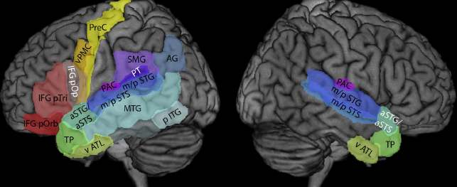
Professor: Above is Fig. 1 from the recent review by Specht (2014). The figure displays all relevant areas that are discussed in his and this review. These are the:

• supramarginal gyrus (SMG, BA 40),
• posterior part of the middle temporal gyrus (MTG, BA 21),
• inferior frontal gyrus, pars opercularis (IFG pOp, BA 44),
• ventral premotor cortex (vPMC, BA 6), and
• precentral gyrus (PreC, BA 4).

Student: Okay, I have taken two puffs from my inhaler. I feel a bit better. So, how do I find a new number for my dyspnea rating score?

Professor: Let me make up a play. First we must have actors and actresses. Below is a listing. For each location, see either the previous figure (on about page 11) from Von Leopoldt and co-workers (2009) or the figure below from Specht, 2012):

• DL (dorsolateral prefrontal cortex, see figure above, to left of vPMC, from Specht)
• SM (SMG, supramarginal gyrus, see figure above from Specht)
• IN (insula, see figure on about page 11 from Von Leopoldt et al.)
• IP (intraparietal sulcus, see figure above, just above SMG, from Specht)
• PM (posterior MTG, middle temporal gyrus, see figure above from Specht)
• VP (vPMC, ventral premotor cortex, see figure above from Specht)
• MC (PreC, precentral (motor) cortex, see figure above from Specht)
• AC (dACC, dorsal anterior cingulate cortex, see figure on about page 11 from Von Leopoldt et al.)
• IF (IFG pOp, inferior frontal gyrus, pars opercularis, see figure above from Specht)

Professor: However, I am not sure whether our brain uses a dialogue format; if it did, the script for a conversation might go like this:

1. Get current SOB state

DL to IN: “What’s a scan of my breathing feel like now?”
IN to DL: “Your body is a bit short-of-breath.”

2. Get current SOB scale descriptor and number

DL to SM: “I have instructions for you to look at your copy of the Borg scale.”
SM to DL: “Last time your rating was ‘Somewhat severe’ with a number of ’4.’”
DL to SM: “Please help IN estimate the present SOB intensity for us.”

SM to IN: “Does SOB feel like ‘somewhat severe’?”
IN to SM: “No. It’s not that intense.”

SM to IN: “How about ‘moderate’?”
IN to SM: “No. That’s still too intense.”

SM to IN: “Do you feel you have ‘slight’ SOB?”
IN to SM: “Yes. It’s just ‘slight’.”

3. Verify SOB scale descriptor and its number

SM to IN: “So, after using the inhaler, your SOB descriptor of ‘slight’ with a number of ’2′ fits okay?
IN to SM: “Yes.”

4. Announce the SOB scale number

SM to DL: “The SOB score for ‘slight’ is ’2.’”

5. Get word for SOB scale number

DL to IP: “What’s the word for ’2′?”
IP to DL: “The non-symbolic label is ‘TWO’”.

6. Assembly phonemes for SOB scale number

DL to IF and PM: “Please get the individual phonemes for the word ‘TWO.’”
IF and PM to DL: “Now the phonemes ‘| tu: |’ are in the auditory working memory.”
DL to VP: “Now prepare an articulatory motor plan for saying ‘| tu: |.’

7. Say phonemes for SOB scale number out loud

VP to MC: “Give the GO signal to execute the motor plan for ‘| tu: |’!”
MC: “Okay you special articulatory motor units for voicing ‘| tu: |’,

• GET READY TO SAY ‘| tu: |’ LOUDLY.
• SET.
• GO!”

8. Get self-feedback while speaking

DL to IN and AC: “Any errors for MC GO action?”
IN to AC: “No interoceptive mismatches; prosody and emotional tone are appropriate!”
AC to IN: “Then, no corrections have to be made!”
IN and AC to DL: “We agree! No errors!”
DL to ALL: “Well done!”

Professor: Maybe that dialogue happened; maybe it didn’t. Something like that surely happened.

Student: Like, I do a lot of ruminating, and your dialogue sounds very familiar to me.

Professor: Thanks. This is the end of the last stage, which basically

• estimates the intensity of breathing discomfort (in this case),
• matches it with an item on a discomfort rating scale,
• retrieves the item number, and
• says the number out loud.

Conclusion

Professor: Now we have come full circle from Part 1. All six stages can be found below in Figure 2 from the review of Davenport (2007):

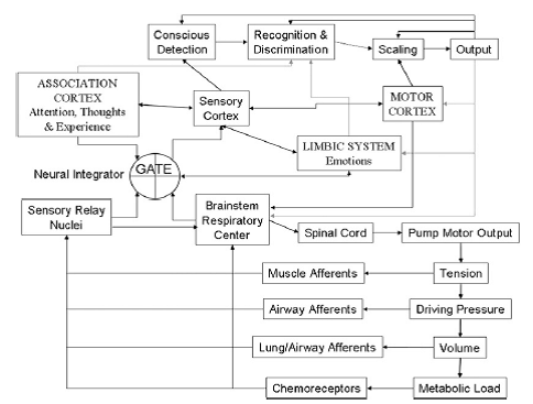
Professor:  The brainstem respiratory center and pump motor output normally keeps driving ventilation and afferents monitors activity as it increases until:

Edit

	Stage	Description in the text	Structure and function in figure
1.	CONTACT!	An alarm signal is sent to the posterior insula.	GATE – Mag-INS searchlight opens sensory gate since it finds significant activity in the reticular thalamus.
2.	SEND OUT ALERT!	Anterior insula and rest of saliency network (SN) receives the alarm, too!	LIMBIC SYSTEM – SN alert system is activated.
3.	FULL ATTENTION!	The SN puts the Central Executive Network (CEN) on the lookout & quiets down the Default Mode Network!	ASSOCIATION CORTEX; Conscious Detection; Recognition & Discrimination – Dyspnea is detected and CEN decides the use of inhaler is okay.
4.	GET READY TO ACT!	Breathing ‘tubes’ want medication via inhaler!	ASSOCIATION CORTEX, Sensory Cortex; Recognition & Discrimination – Visually finds location of inhaler and creates a motor plan to get it and use it.
5.	ACT!	Go get inhaler and use it!	ASSOCIATION CORTEX, Sensory Cortex; Recognition & Discrimination; MOTOR CORTEX – Premotor cortex releases inhibition of motor plan.
6.	COMMUNICATE!	Let others know how well the medication is working!	Recognition & Discrimination; Scaling; Output – Estimates the SOB intensity, prepares the articulatory motor plan, and does it.

Professor: I am looking forward to applying these six stages to other sensations, for example, perceived effort and physical fatigue.

Take Home: Predict Outcomes and Notice Mismatches:

• CONTACT!
• SEND OUT ALERT!
• FULL ATTENTION!
• GET READY TO ACT!
• ACT!
• COMMUNICATE!

Next: Perceived Effort: how do we predict (produce) and notice mismatches (estimate).

 References

Borg, G. (1982) Psychophysical basis bases of exertion. Med Sci Sports Med 14: 377-381.

Borg, G. (1998) Borg’s Perceived Exertion and Pain Scales. Champain, IL: Human Kinetics.

Borovsky A, Elman J, Fernald A. (2012) Knowing a lot for one’s age: Vocabulary skill and not age is associated with anticipatory incremental sentence interpretation in children and adults. J Exp Child Psychol 112: 417–436. doi:10.1016/j.jecp.2012.01.005.

Carter R, Frith C. (2010) Mapping the Mind. Oakland, CA: University of California Press.

Davenport PW. (2007) Chemical and mechanical loads: What have we learned? In: O’Donnell DE, Banzett RB, Carrieri-Kohlman V, Casaburi R, Davenport PW, Gandevia SC, Gelb AF, Mahler DA, Webb KA. Pathophysiology of Dyspnea in Chronic Obstructive Pulmonary Disease: A Roundtable. Proc Am Thorac Soc 4: 147–149.

Dikker S, Pylkkanen L. (2013) Predicting language: MEG evidence for lexical preactivation. Brain Lang 127(1):55-64. doi: 10.1016/j.bandl.2012.08.004.

Hickok, G, Poeppel D. (2007) The cortical organization of speech processing. Nature Rev Neurosc 8: 393–402.

Kahn D, Hobson JA. (2005) State-dependent thinking: A comparison of waking and dreaming thought. Conscious Cogn 14: 429-438.

Kotz SA, Schwartze M. (2010) Cortical speech processing unplugged: A timely subcortico-cortical framework. Trends Cogn Sci 14: 392–399

Langers DRM, van Pijk P. (2012) Mapping the tonotopic organization in auditory cortex with minimally salient acoustic stimulation.  Cereb Cortex 22: 2024-2038.

Menon V, Uddin UQ. (2010) Saliency, switching, attention, and control: A network model of insula function. Brain Struct Funct 214: 655–667. doi:10.1007/s00429-010-0262-0.

Petersen SE, Fox PT, Posner MI, Mintun M, Raichle ME. (1988) Positron emission tomographic studies of the cortical anatomy of single-word processing. Nature 331: 585–589.

Price CJ. A review and systhesis of the first 20 years of PET and fMRI studies of heard speech, spoken language and reading. NeuroImage 62: 816-847.

Rauschecker JP, Scott SK. (2009) Maps and streams in the auditory cortex: Nonhuman primates illuminate human speech processing. Nat Rev Neurosc 12:718-725.

Specht K. (2014) Neuronal basis of speech comprehension. Hearing Research 307: 121.135. DOI.org/10.1016/j.heares.2013.09.011.)

Tyler LK, Cheung TPL, Devereux BJ, Clarke A. (2013) Syntactic computations in the language network: Characterizing dynamic network properties using representational similarity analysis. Front Psych doi: 10.3389/fpsyg.2013.00271.

Tyler LK, Marslen-Wilson, WD. (2008) Phil. Trans R Soc B 363: 1037–1054. doi:10.1098/rstb.2007.2158

von Leopoldt A, Sommer T, Kegat S, Baumann HJ, Klose H, Dahme B, Büchel C. (2009) Dyspnea and pain share emotion-related brain network. NeuroImage 48:  200–206. doi:10.1016/j.neuroimage.2009.06.015.

Weiser PC, Mahler DA, Ryan KP, Hill KL, Greenspon LW. Clinical assessment and management of dyspnea. In: Pulmonary rehabilitation: Guidelines to success. Hodgkin, J, Bell CW, eds. Philadelphia: Lippincott 1993, 478-511.