Student: Wow, was I ever slipping and sliding, just trying to walk outside. It was a street with patches of ice: step, step, slide, step, sliiiide, ….

Professor: My walking was off today, too. I was limping from sore knee like like walking in a wooden leg: step, thump, step, thump, ….

Student: I noticed I was got ‘off balance’ but without thinking I never fell down.

Professor: Hmm. We could be correcting for perceived differences, i.e., errors, from where we were supposted to be walking and where we were actually walking.

Malone, Bastian, & Torres-Oviendo (2012) recently studied walking errors in detail. Below is their Figure 1 that illustrates how this errors signal may happen and could be used to make a smooth adaptive transition from a sudden change, i.e., perturbation, while walking:

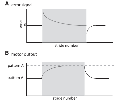
Fig. 1. Schematic of error signal and motor output. Shaded region represents the adaptation period. A: Parameters quantifying error are perturbed early in adaptation and decrease throughout adaptation. They also show the opposite perturbation in deadaptation. B: Motor outputs exhibit a smooth change from a set pattern A to a new value during adaptation (pattern A’), set by the environmental conditions. They also must be actively deadapted with a smooth transient from pattern A’ to pattern A when environmental conditions change back to the original state. [Emphases added.]

Student: How can we measure the error between what is expected and what is actual for walking?

Professor: What did Malone and her co-investigators utilize for measuring walking? They used gait parameters as shown below in their Figure 2:

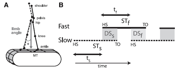
Fig. 2. Definitions of parameters. A: Marker diagram for experiments 1 and 2 with limb angle convention shown. MT, 5th metatarsal head. By convention, positive limb angles represent when the ankle is in front of the hip (flexion) and negative angles when it is behind (extension).B: Schematic defining temporal parameters of locomotion during normal, symmetric walking. Time is represented along the horizontal axis, with time increasing from left to right. HS, time at heel-strike; TO, time at toe-off. Solid and dashed lines represent stance time periods (ST) for the slow (ST_s) and fast (ST_f) legs, respectively. White areas between these lines represent swing time periods (i.e., time intervals from TO to HS). Shaded areas indicate when both feet are on the ground, defined as double support periods (i.e., overlap in stance time for both legs); DS_s and DS_f are slow and fast double support periods, respectively. Slow and fast step timings (t_s and t_f) are defined as the time between consecutive heel-strikes. [Emphases added.]

Professor: The legend for their Fig. 2 shows these important parameters. The Stance Time for the ‘slow’ leg (ST_s) is from Heal Strike (HS) to Toe Off (TO) of the slow limb; vice versa for the ‘fast’ leg Stance Time (ST_f). Double Support for the slow leg (DS_s) begins at heel strike for the fast leg and lasts until toe-off for slow limb; vice versa for the fast leg. During Stride Time for the slow leg, its Step Time (t_s) lasts to the beginning of Double Support; vice versa for the fast leg (t_f). Stride Time (Tstride) for either leg was the difference in time from heel strike to the subsequent heel strike.

Malone and colleagues (2012) hypothesized that if adapatation in timing coordination, i.e. temporal coordination, occurred, then a change in double support might happen. So, they:

“…defined the temporal motor error (et) as the difference in double support times:

e_t = DS_s – DS_f

where DS_s and DS_f  are the double support times for the “slow” and “fast” limbs, respectively.”

Professor: To minimize the temporal motor error, they suggested that:

“…during split-belt walking the temporal motor output approaches a new steady state, Tdesired, specified by the difference in stance times in the asymmetric environment.  Accordingly, we defined Tout as the difference in slow and fast step times (ts and tf, respectively) normalized by the stride time (Tstride):

Tout = (t_s – t_f)/Tstride = (t_s – t_f)/(t_s + t_f)

The full derivation of Tout is provided in APPENDIX A. We also defined Tdesired, or the value that Tout could approach to equalize double support times, as:

Tdesired = (ST_s – ST_f)/Tstride

The full derivation of Tdesired is also given in APPENDIX A.”

Professor: This temporal motor output is calculated from the step times is shown at the top of their Fig. 3:

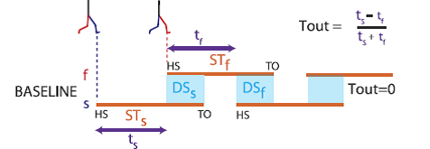
Fig. 3. Schematic of temporal changes throughout adaptation. Stick figures show limb configuration at heel-strike for the fast (red) and slow (blue) limbs. Stance periods are shown by orange lines. Double support periods are represented by the shaded blue squares. Slow and fast step timings are shown by the purple arrows. Temporal motor output (Tout) is a normalized difference of step timings. When belts are tied during baseline walking, a temporal motor output of zero (equal purple arrows) and equal double support periods (blue regions) are apparent. [Emphases added.]

Student: Then a timing error can be corrected by increasing the motor output in the time domain as an increased difference in step times of the limbs.

Professor: Yes. Now let’s look at what happened to the step times as shown in their Fig. 4:

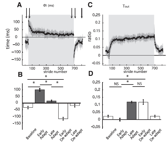
Fig. 4. Group averages of temporal parameters throughout experiment 1. Adaptation period is represented by shaded area. Arrows represent time correspondence between bar graphs and group average curves; the first arrow corresponds to the first epoch (baseline), and so forth. A: Stride-by-stride time course of the temporal error (e_t) characterized by the double support difference. e_t follows the characteristic time course of a motor error: large values during early adaptation, error reduction as subjects adapt, and aftereffects during early deadaptation that are actively washed out. B: Key epochs are shown for the error parameter double support difference. Abrupt transitions in e_t values are observed when the environmental conditions change (e.g., tied to split). This is indicated by the significant differences between baseline and early adaptation and those between late adaptation and early deadaptation. Also, subjects adapted by the significant decrease in e_t from early to late adaptation and stored as indicated these changes as shown by the aftereffects demonstrating the opposite asymmetry in early deadaptation. C: Stride-by-stride time course of the temporal motor output (Tout). Tout follows the characteristic time course of motor outputs. Contrary to the temporal error time course, the temporal motor output smoothly changes from zero in baseline (tied) walking to values greater than zero during adaptation, and smoothly changes back to zero during deadaptation when the belts run in tied mode. D: Key epochs are shown for Tout. Two important features characterizing the behavior of motor outputs are observed. First, there are smooth transitions between tied and split conditions as shown by the similarity in Tout values from baseline to early adaptation and from late adaptation to early deadaptation. Second, there is a statistical increase in Tout values from early to late adaptation. [Emphases added.]

Student: Aha! Look at those curves. The time course for changes in the calculated error signal is very clear.

Professor: And more importantly, the increase in calculated temporal motor output appears to be closely associated with the dropping error signal approaching zero.

Student: Then the mirror opposite happens during deadaptation.

Professor: So, that’s took place in the time dimension, i.e., ‘when’. Let me use their conclusion from the bottom of the Fig. 4 legend:

“Two important features characterizing the behavior of motor outputs are observed. First, there are smooth transitions between tied and split conditions as shown by the similarity in T_out values from baseline to early adaptation and from late adaptation to early deadaptation. Second, there is a statistical increase in T_out values from early to late adaptation.” [Empases added]

Professor: What happens ‘where’ we step, i.e., in the spatial placement dimension. That is shown below in their Figure 5:

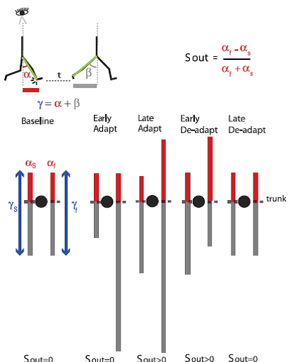
Fig. 5. Schematic of spatial changes occurring throughout adaptation. Stick figures at top show the sagittal view of someone walking on the treadmill. The limb angle at heel-strike (i.e., α) is shown at a time period t before the limb angle is at toe-off (i.e., β). Eye icon indicates that diagrams below the sagittal schematic represent the bird’s-eye view of the subject stepping on the treadmill. Lines in the bird’s-eye view are projections of limb motions during stance at different points in the experimental paradigm. Trunk position is represented by black circles. Red and gray lines represent limb axis projection at angles α and β. Blue arrows represent the range of motion for a single limb’s stride, which depends on the limb excursion (angle γ). In baseline, the proportion of the limb-forward placement with respect to its entire movement is the same for both legs. This symmetry is disrupted when placing the legs at the same angle α [spatial motor output (Sout) = 0] during early adaptation. Thus subjects adapt their limb-forward placement to reestablish symmetry in proportions of limb-forward placement with respect to the entire limb motion in both legs during late adaptation. In deadaptation, the belts are tied to the same speed. The nervous system still attempts to maintain the new spatial motor output in early adaptation, but now the limbs’ spatial error (limb-forward placement with respect to the entire movement) is asymmetric in the opposite direction. By the end of deadaptation, Sout returns back to zero and walking is similar to what is seen at baseline.  [Emphases added.]

Professor: Note carefully how their legend explans the limb angles at heel strike, i.e., α, and from heel strike to toe-off of the same limb, i.e., γ. From these they:

“… quantify  this [oscillation] for each limb by computing an angular ratio (r), which indicates the proportion of limb flexion compared to the entire range of motion of the leg:

r_s =α_s/γ_s and r_f = α_f/γ_f

Here α_s and α_f are the limb angles at heel-strike of the slow and fast legs, respectively (see Fig. 5). Similarly, γ_s and γ_f are the limb angles from heel-strike to toe-off of the slow and fast legs, respectively. In other words, γ_s and γ_f values quantify the entire range of motion for each leg, or total amplitude of oscillation for each leg during one stride (see Fig. 5). Note that limb angle is defined here as the angle between a vertical line and the vector from the hip to the ankle on an x-y plane (Fig. 2A); by convention, it is positive when the ankle is in front of the hip (flexion) and negative behind (extension). defined the spatial error. …”

“Our prior work has also shown that people adapt their center of oscillation values to be equal on the two legs (Malone and Bastian 2010). We therefore defined the spatial error (es) as the difference in angular ratios:

e_s = r_s – r_f

We hypothesized that the spatial motor output (S_out) is adapted to recover spatial gait symmetry. We further hypothesized that Sout is a function of the limb angle (α) at heel-strike,

… We defined S_out as the difference between fast and slow limb angles at heel-strike (α_f and α_s, respectively) normalized by their sum:

S_out = (α_f – α_s) / (α_f + α_s)

The full derivation of this is provided in APPENDIX B. We also defined Sdesired, or the value that the spatial motor output could approach for angular ratio symmetry, as:

S_desired = (γ_f – γ_s) = (γ_f + γ_s)

The full derivation of S_desired is also given in APPENDIX B.

In conclusion, we propose that the spatial motor output is determined by the limbs’ orientation at heel-strike. We further suggest that during split-belt walking the spatial motor output approaches a new steady state, S_desired, specified by the difference in the limbs’ range of motion in the asymmetric environment. This is accomplished in order to minimize the spatial motor error (e_s) characterizing the asymmetry in orientation of the limbs’ oscillations that subjects experience during split-belt walking.”

Professor: The bird’s eye view of the walker at the bottom of Figure 5 shows the adaptation and deadaptation for split-belt locomotion. Orange bars are the angle from vertical at heel-strike in each condition, and blue bars are the angle for the entire stride in each epoch

Now let’s see what happens as the participants walk as shown in their figure 6:

 

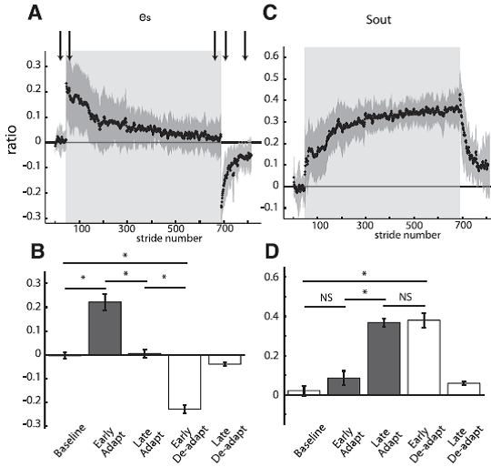
Fig. 6. Group averages of spatial parameters throughout experiment 1 are shown similarly to the temporal parameters in Fig. 4. Adaptation period is represented by shaded area. Arrows represent time correspondence between bar graphs and group average curves; the first arrow corresponds to the first epoch (baseline), and so forth. A: Stride-by-stride time course of the spatial error (e_s) characterized by the difference in angular ratios. B: Key epochs are shown for the e_s. C: Stride-by-stride time course of the spatial motor output (Sout) characterized by a normalized difference in limb angles at heel-strike. D: Key epochs are shown for the Sout. [Emphases added.]

Student: Again; the very rapid error resulting from ‘splitting’ the belts is very impressive! Compared to the timing changes, the positioning adaptation seems much slower.

Professor: I agree. Otherwise, the adaptation and deadaptation are very similar.  S_out is like S_out as a parameter to characterize motor ouput change to reduce spatial error.

Now let’s find out the differences between adaptive changes in the timing and in the placing of the limbs compared to the parameters they proposed to measure re-establish symmetry, T_desired and S_desired. These are shown below in their Figure 7:

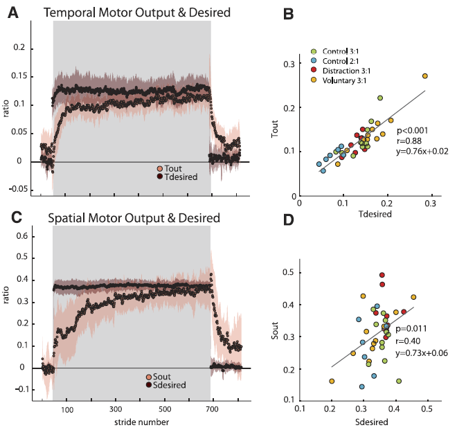
Fig. 7. Temporal and spatial motor outputs with their respective desired values (derivation in METHODS and APPENDIXES A and B, respectively). Adaptation period is represented by shaded region. Group average plots for the Distraction group are shown with shaded standard error regions in A (temporal) and C (spatial). Note that the spatial (Sdesired) and temporal (Tdesired) desired values change immediately upon the split-belt perturbation, while the motor outputs change on a stride-by-stride basis. On average, by the end of adaptation, the motor outputs approached the desired values. B and D: Scatterplots of each subject’s Tdesired vs. Tout (B) and Sdesired vs. Sout (D). Each group in experiment 1 is classified in different colors. Only subjects from the Control group in experiment 2 are also included in this analysis. Although regression results show that “desired” values are a good predictor of the steady-state values reached by motor outputs, the temporal correlation coefficient is larger than the spatial coefficient. This suggests that the temporal parameter is more tightly controlled in individual subjects. [Emphases added.]

Professor:

“We proposed that the temporal motor output would approach T_desired to reestablish temporal symmetry (e_{t =} 0) and the spatial motor output would approach S_desired to reestablish spatial symmetry (e_{s =} 0). We observed that in late adaptation the averaged motor outputs approached the “desired” temporal (T_desired) and spatial (S_desired) parameters for symmetric gait (Fig. 7A, temporal; Fig. 7C, spatial).”

 

“We observed that T_desired and S_desired do not adapt, and instead change rapidly when experimental conditions change (i.e., rapid jump from baseline to early adaptation and again from late adaptation to early deadaptation). Scatterplots of individual subjects’ desired values versus motor output in late adaptation (i.e., last 10 strides) are shown for temporal and spatial parameters in Fig. 7, B and D, respectively.”

 

A regression was performed, and there was a significant correlation of the respective desired parameters for both temporal and spatial outputs (temporal P < 0.01 and spatial P = 0.01). … Although both motor outputs could be significantly predicted by their respective desired values, there was a much stronger correlation for the temporal parameters (r = 0.88) as opposed to the spatial parameters (r = 0.40). These results suggest that it might be more important for subjects to achieve temporal symmetry than spatial symmetry.”

S

P

Spatial Hold Figure 8:

 

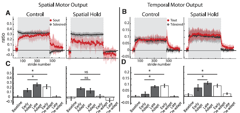
Fig. 8. Group averages and standard errors of Sout, Sdesired, Tout, and Tdesired for Control (N  7) and Spatial Hold (N = 7) groups. A: Stride-by-stride time course of Sout and Sdesired for both groups. Adaptation period is represented by shaded area in gray. Spatial motor output adapted normally for the Control group, while the Spatial Hold group was prevented from adapting the spatial motor output. B: Stride-by-stride time course of Tout and Tdesired for both groups. Adaptation period is represented by shaded area in gray. Although Sout was not adapted in the Spatial Hold group, Tout adapted normally in this group. This suggests that the adaptation of temporal and spatial motor outputs is dissociable. C: Statistical analysis on the first 10 strides of Sout for key epochs in the experimental paradigm. A significant change from early to late adaptation was found for the Control but not the Spatial Hold group. Also, significant storage from baseline to early deadaptation was found for the Control but not the Spatial Hold group. D: Statistical analysis on the first 10 strides of Tout for key epochs in the experimental paradigm. In both groups Tout adapted normally: there were significant differences between early adaptation and late adaptation and between baseline and early deadaptation. [Emphases added.]

Professor:

“Results from experiment 2 indicate that the temporal motor output can be adapted during split-belt walking when the adaptation of spatial motor output is consciously prevented. This finding signifies that the spatial and temporal adaptations are dissociable. Group averages of spatial and temporal motor outputs of subjects in the Control and Spatial Hold groups are shown in Fig. 8. We observed that S_out in the Spatial Hold group does not change during adaptation, whereas there was a clear change in S_out during adaptation in theControl group (Fig. 8A). This is indicated by the significant interaction between group and epoch [F(4,38) = 5.13, P < 0.01]. To verify that the Spatial Hold group did not adapt their leg configuration, we tested for epoch effects for the ankle and knee angles and found that they did not change significantly across epochs [F(4,24) = 1.03, P = 0.41 for ankle; F(4,24) = 1.37, P = 0.27 for knee]. We found that the Control group displayed a significant change in S_out from early to late adaptation (P < 0.001), while the Spatial Hold group did not (P = 0.22). Consequently, the new stepping pattern learned during split-belt walking was stored in the Control group, as indicated by the significant differences between baseline and early deadaptation S_out values (P < 0.01), but not in the Spatial Hold group (P  0.23).

Conversely, while there were differences in the adaptation of spatial motor outputs across the Control and Spatial Hold groups, both groups adapted their temporal motor outputs similarly [F(4,48) = 1.11, P = 0.36; Fig. 8, B and D]. We observed that there was a significant effect of epoch in both groups [F(4,48) = 19.44, P < 0.001]. In both groups, T_out had significantly different values between early and late adaptation (P < 0.001) and there were significant differences between baseline and early deadaptation (P < 0.001). This indicates that in both groups the changes in T_out with adaptation were stored (Fig. 8D). In conclusion, we demonstrated with this experiment that subjects can adapt their temporal motor output without adapting their spatial motor output — dissociating temporal and spatial adaptation of locomotion.

Temporal hold

Additionally, we attempted to prevent the temporal motor output from adapting but found that this was not as easily accomplished as clamping the spatial adaptation. Subjects were provided with an auditory cue of when to land their feet—a symmetric rhythm (i.e., T_out = 0). However, we found that healthy adults were not able to prevent their temporal motor output from adapting.

DISCUSSION

“Here we describe two parameters that characterize temporal and spatial motor outputs for locomotion. The temporal motor output is a normalized difference between step timings (i.e., stepping rhythm), while the spatial motor output is a normalized difference between limb angles at heel-strike (i.e., stepping pattern). Both these motor outputs adapt in order to regain temporal and spatial symmetry. Importantly, in this study we were able to dissociate the adaptation of temporal and spatial control. Although the nervous system typically adapts both temporal and spatial parameters, we found that there is more consistent and tighter control of the temporal motor output, suggesting a priority in the adaptation of timing. Moreover, this tighter control of the temporal motor output could also suggest distinct neural structures that control more precisely the adaptation of the temporal control versus the spatial control of stepping in locomotion. In sum, these results suggest that there are separate neural mechanisms that control temporal and spatial locomotion parameters.

“Numerous parameters could theoretically capture motor output behavior in walking, particularly since it is a multisegmental and bilateral cyclical movement. … Furthermore, we think that heelstrike is important for the nervous system to control in a feedforward manner, whether it is the duration between heelstrikes or the limb orientation at heel-strike. … Since motor outputs have been suggested to represent feedforward adjustments of the nervous system (Smith et al. 2006), this leads us to believe that the temporal and spatial control of heel-strike utilizes feedforward mechanisms to update the subsequent heel-strike.

“Although there is an important contribution of the spinal cord, brain stem, and motor cortex in the control of locomotion (Bretzner and Drew 2005; Hayes et al. 2009; Le Ray et al. 2011), the cerebellum is important for the adaptation of the locomotor pattern. The cerebellum is believed to have a role in monitoring errors and updating the motor outputs (Shadmehr and Krakauer 2008), and, not surprisingly, the cerebellum has been shown to be essential for many forms of motor adaptation (Criscimagna-Hemminger et al. 2010; Lewis and Zee 1993; Maschke et al. 2004; Tseng et al. 2007), including split-belt walking adaptation (Morton and Bastian 2006). Locomotor adaptation likely involves the interaction between the cerebellum and cortical or brain stem structures; however, we know that cerebral motor areas are less essential for this adaptation in humans, since individuals with cerebral stroke and hemiparesis can adapt normally (Choi et al. 2009; Reisman et al. 2007, 2009). Work in the cat shows that spinal circuits alone can produce rhythmic stepping patterns on a split-belt treadmill (Forssberg et al. 1980). However, without cerebellar integrity, spinal circuits cannot adapt the locomotor pattern to restore spatial and temporal symmetry (Yanigahara and Kondo 1996). Therefore, we felt it was important to determine that the errors and motor outputs described here were neural inputs/outputs of the cerebellum. For spatial coordination, neural recordings in cats have shown that signals of lower limb length and orientation during locomotion are carried in the dorsal spinocerebellar tract (Bosco and Poppele 2001). Additionally, it has been demonstrated that neurons in the dorsospinocerebellar tract respond differently to bipedal movements compared with ipsilateral movements (Poppele et al. 2003), suggesting that the spatial relationship between both limbs is important to the nervous system. With regard to temporal coordination, additional neural recording studies in cats have found that cerebellar discharges from Purkinje cells are most active at the time of foot contact (Apps and Lidierth 1989; Apps et al. 1995), possibly indicating the importance of this event in the gait cycle. Taken together, these results suggest that some of the essential elements of our model are accessible by the cerebellum for the purposes of adapting movements to predicable perturbations. section on “Separation of temporal and spatial control of locomotion.”

“Our findings show separate control of the temporal and spatial parameters of locomotion in this adaptive task. Some of our previous studies have treated these parameters as if they were controlled by overlapping neural systems and would therefore adapt together (Choi and Bastian 2007). However, our more recent work suggests that temporal and spatial parameters may be controlled, and therefore adapted, separately. Children with hemispherectomies, where one half of the cerebrum is removed, adapted their step symmetry but not their double support errors (Choi et al. 2009). Additionally, we have seen that experimental conditions such as consciously controlling the gait or dual-tasking while walking affected the adaptation rate in spatial parameters, but temporal parameters remained unaffected (Malone and Bastian 2010). In that study, we found that the temporal coordination was adapted at a rate almost two times faster than the spatial coordination, even under “control” conditions in which we asked subjects to “just walk.” Here we see similar trends: the spatial parameters take longer to adapt than the temporal parameters (compare spatial and temporal motor outputs in Figs. 4C and 6C). However, in our prior studies spatial and temporal parameters always adapted, just at different rates. While these findings led us to hypothesize separate control and distinct neural substrates of spatial and temporal control of locomotion, this study allowed us to completely dissociate the two. From our direct investigation into the independence of parameters, we found that subjects could consciously prevent their spatial motor output from adapting while the temporal motor output was unaffected.

“We also observed that subjects tended to reach temporal symmetry at the adapted state more often than spatial symmetry, thereby suggesting tighter control of the temporal coordination in this locomotor task. Each motor output (temporal and spatial) tended to approach a “desired” value by the end of adaptation that we derived mathematically, using specific error parameters (see METHODS, APPENDIXES A and B). For temporal coordination, the “desired” parameter was a relationship between stance times (Fig. 3, orange lines). In space, the “desired” value was a relationship between the limb ranges of motion (Fig. 5, blue arrows). Not only did group average curves for the spatial and temporal motor outputs approach the group average “desired” values, but these relationships held true with individual subjects as well. When we regressed the “desired” parameter with the final plateau of the motor output for both spatial and temporal coordination, we found significant positive correlations. Although this result was found for both temporal and spatial coordination, the temporal relationship was more tightly controlled than the spatial relationship (i.e., larger correlation coefficients). In other words, the temporal motor output was more likely to reach the “desired” value (normalized difference of stance times) than the spatial counterparts. While this suggests that temporal asymmetries are smaller than spatial asymmetries in the adapted state, it is difficult to directly compare the temporal and spatial features because temporal and spatial coordination are expressed in different units in this analysis. Future studies will investigate how temporal and spatial motor outputs can combine in order to equalize steps.

“Additionally, we attempted to prevent the temporal motor output from adapting but found that this was not as easily accomplished as clamping the spatial adaptation. Subjects were provided with an auditory cue of when to land their feet—a symmetric rhythm (i.e., Tout  0). However, we found that healthy adults were not able to prevent their temporal motor output from adapting. We hypothesize that this could be due to a number of reasons. First, subjects may not be able to consciously prevent the temporal motor output from adapting under split-belt conditions (i.e., temporal control was harder to influence with conscious efforts; Malone and Bastian 2010). Second, the temporal changes induced by a speed ratio of 2:1 on the split-belt treadmill are small (between 100 and 150 ms). It is possible that while both the subjects and experimenter perceived subjects landing on the time specified by the auditory cue, they do not have the resolution to make conscious perceptions and adjustments on that timescale. Future work will be done to investigate whether different types of feedback on timing control will allow healthy adults to consciously adjust their locomotor timing. “This more stringent control of timing agrees with previous studies in our lab in which we found that temporal control was invariant to conscious efforts (Malone and Bastian 2010) and training structure (Malone et al. 2011). Additionally, temporal adaptation was found to be fully developed by the age of 3, while spatial adaptation continued to develop well into adolescence (Vasudevan et al. 2011), leading us to believe that temporal control is more automatic and perhaps depends more heavily on subcortical circuits.”

S: Wow

 

Take Home: Automatic, smooth even-sided pattern
Monitored and modified by cerebellum and basal ganglia

 

References

Malone etal 2012

Last updated: 4 Apr 2013